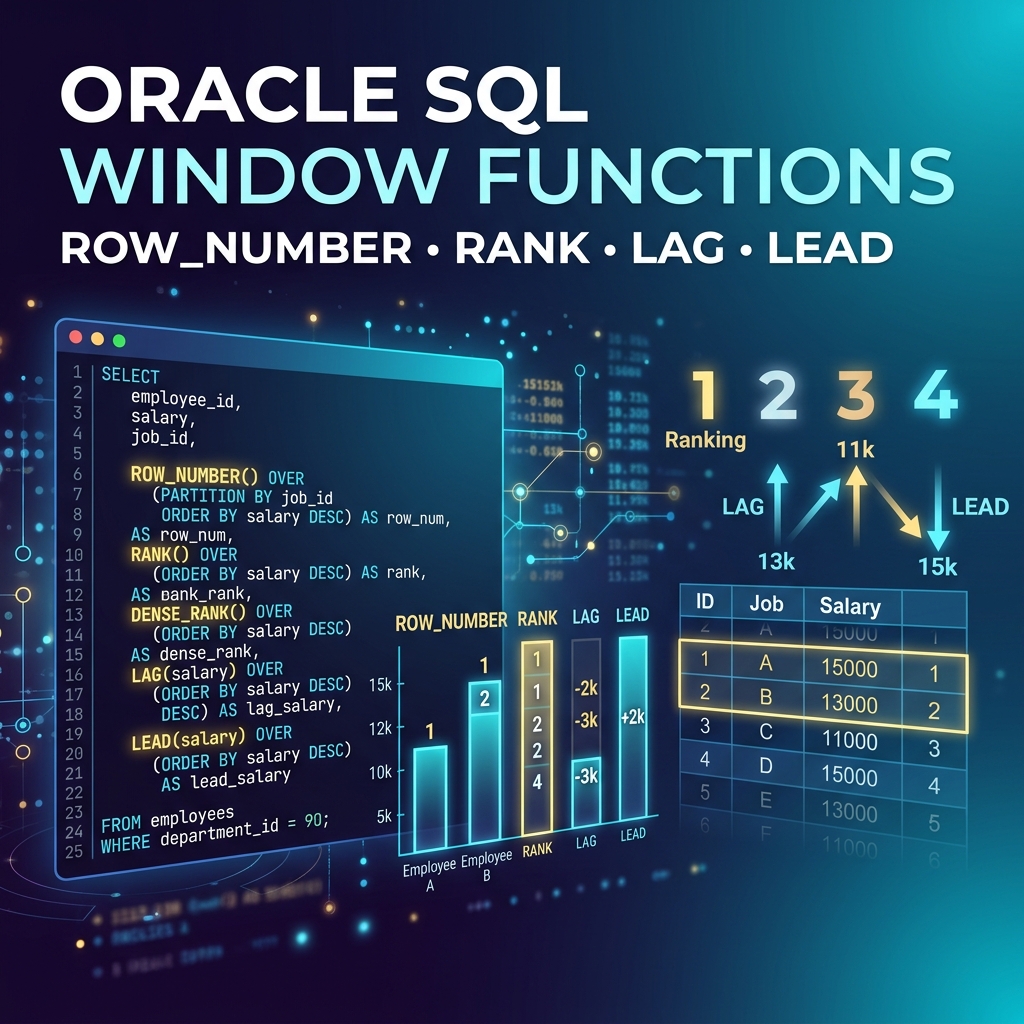
Oracle SQL Window Functions: A Complete Practical Guide

Window functions are one of the most powerful and underused features in Oracle SQL. Once you understand them, you will find yourself reaching for them constantly — for rankings, running totals, moving averages, comparing rows to previous or next rows, and much more.

In this guide, we cover the most important Oracle window functions with real, working examples so you can immediately apply them to your own queries.

What Is a Window Function?

A window function performs a calculation across a set of rows that are related to the current row — a “window” of data. Unlike GROUP BY which collapses rows into a single result, window functions preserve all individual rows while adding an aggregated or analytical value alongside each one.

The key syntax component is the OVER() clause, which defines the window:

function_name(expression) OVER (
  [PARTITION BY column1, column2, ...]
  [ORDER BY column3 ASC|DESC]
  [ROWS|RANGE BETWEEN ... AND ...]
)

ROW_NUMBER, RANK, and DENSE_RANK

These three functions assign sequential numbers to rows based on an ORDER BY clause.

SELECT 
  employee_id,
  last_name,
  department_id,
  salary,
  ROW_NUMBER()  OVER (PARTITION BY department_id ORDER BY salary DESC) AS row_num,
  RANK()        OVER (PARTITION BY department_id ORDER BY salary DESC) AS rnk,
  DENSE_RANK()  OVER (PARTITION BY department_id ORDER BY salary DESC) AS dense_rnk
FROM employees
ORDER BY department_id, salary DESC;

The difference between them matters when there are ties:

Employee	Salary	ROW_NUMBER	RANK	DENSE_RANK
Smith	9000	1	1	1
Jones	8000	2	2	2
Brown	8000	3	2	2
Davis	7000	4	4	3

Use ROW_NUMBER when you need unique sequential numbers regardless of ties. Use RANK when ties should receive the same rank with a gap after. Use DENSE_RANK when ties share a rank but there is no gap — the next rank is always the next integer.

Practical Use: Top-N Per Group

One of the most common real-world uses of ROW_NUMBER is finding the top N records per group. For example, the top 3 earners per department:

SELECT department_id, last_name, salary
FROM (
  SELECT 
    department_id,
    last_name,
    salary,
    ROW_NUMBER() OVER (PARTITION BY department_id ORDER BY salary DESC) AS rn
  FROM employees
)
WHERE rn <= 3
ORDER BY department_id, salary DESC;

This pattern — window function in a subquery, filter on the result — is used constantly in reporting queries.

Running Totals with SUM OVER

SELECT 
  order_date,
  order_amount,
  SUM(order_amount) OVER (ORDER BY order_date) AS running_total,
  SUM(order_amount) OVER (
    PARTITION BY TO_CHAR(order_date, 'YYYY-MM')
    ORDER BY order_date
  ) AS monthly_running_total
FROM orders
ORDER BY order_date;

The first SUM gives a cumulative total across all time. The second resets each month (due to the PARTITION BY on year-month). Both are calculated in a single query pass.

Moving Averages with ROWS BETWEEN

The window frame clause (ROWS BETWEEN) gives you fine-grained control over which rows are included in the calculation:

SELECT 
  sale_date,
  daily_sales,
  AVG(daily_sales) OVER (
    ORDER BY sale_date
    ROWS BETWEEN 6 PRECEDING AND CURRENT ROW
  ) AS seven_day_moving_avg
FROM daily_sales_summary
ORDER BY sale_date;

This calculates a 7-day moving average: the current row plus the 6 preceding rows. No self-joins or complex subqueries needed.

LAG and LEAD: Accessing Adjacent Rows

LAG and LEAD let you reference the previous or next row's value within the same result set. This is invaluable for period-over-period comparisons:

SELECT 
  sale_month,
  total_sales,
  LAG(total_sales, 1, 0)  OVER (ORDER BY sale_month) AS prev_month_sales,
  LEAD(total_sales, 1, 0) OVER (ORDER BY sale_month) AS next_month_sales,
  total_sales - LAG(total_sales, 1, 0) OVER (ORDER BY sale_month) AS month_over_month_change,
  ROUND(
    (total_sales - LAG(total_sales, 1, 0) OVER (ORDER BY sale_month)) 
    / NULLIF(LAG(total_sales, 1, 0) OVER (ORDER BY sale_month), 0) * 100, 
    2
  ) AS pct_change
FROM monthly_sales
ORDER BY sale_month;

The third parameter to LAG/LEAD is the default value when there is no previous/next row (first and last rows). Using 0 instead of NULL keeps calculations clean.

FIRST_VALUE and LAST_VALUE

These functions return the first or last value in the window frame — great for anchoring comparisons against a baseline:

SELECT 
  employee_id,
  last_name,
  department_id,
  salary,
  FIRST_VALUE(salary) OVER (
    PARTITION BY department_id 
    ORDER BY salary DESC
  ) AS highest_dept_salary,
  LAST_VALUE(salary) OVER (
    PARTITION BY department_id 
    ORDER BY salary DESC
    ROWS BETWEEN UNBOUNDED PRECEDING AND UNBOUNDED FOLLOWING
  ) AS lowest_dept_salary,
  ROUND(salary / FIRST_VALUE(salary) OVER (
    PARTITION BY department_id ORDER BY salary DESC
  ) * 100, 1) AS pct_of_max
FROM employees
ORDER BY department_id, salary DESC;

Note the ROWS BETWEEN UNBOUNDED PRECEDING AND UNBOUNDED FOLLOWING on LAST_VALUE. Without it, LAST_VALUE defaults to the current row's frame which gives unexpected results — a common gotcha.

NTILE: Dividing Rows into Buckets

NTILE divides rows into a specified number of equally-sized groups (buckets), numbered from 1 to N:

SELECT 
  employee_id,
  last_name,
  salary,
  NTILE(4) OVER (ORDER BY salary) AS salary_quartile
FROM employees
ORDER BY salary;

Employees are divided into four salary quartiles. NTILE(10) creates deciles, NTILE(100) creates percentiles. This is the easiest way to segment data into performance bands or cohorts.

PERCENT_RANK and CUME_DIST

SELECT 
  last_name,
  salary,
  PERCENT_RANK() OVER (ORDER BY salary) AS pct_rank,
  CUME_DIST()    OVER (ORDER BY salary) AS cumulative_dist
FROM employees
ORDER BY salary;

PERCENT_RANK returns a value from 0 to 1 representing where the row falls relative to all other rows. CUME_DIST returns the proportion of rows with a value less than or equal to the current row. These are useful for statistical analysis and percentile reporting.

Combining Multiple Window Functions

The real power comes from combining multiple window functions in a single query:

SELECT 
  d.department_name,
  e.last_name,
  e.salary,
  RANK()       OVER (PARTITION BY e.department_id ORDER BY e.salary DESC) AS dept_rank,
  SUM(e.salary) OVER (PARTITION BY e.department_id) AS dept_total_payroll,
  ROUND(e.salary / SUM(e.salary) OVER (PARTITION BY e.department_id) * 100, 1) AS pct_of_payroll,
  AVG(e.salary) OVER (PARTITION BY e.department_id) AS dept_avg_salary,
  e.salary - AVG(e.salary) OVER (PARTITION BY e.department_id) AS vs_dept_avg
FROM employees e
JOIN departments d ON e.department_id = d.department_id
ORDER BY d.department_name, e.salary DESC;

This single query shows every employee with their rank in the department, the department's total payroll, their percentage of that payroll, and how their salary compares to the department average. In older SQL, this would require multiple subqueries or self-joins.

Performance Considerations

• Window functions are generally efficient — Oracle processes them in a single pass through the data for most cases
• Indexes help when PARTITION BY or ORDER BY columns are indexed
• Avoid unnecessary PARTITION BY — If the window spans all rows, leave PARTITION BY out
• Check execution plans — Look for WINDOW SORT operations and ensure they are not performing excessive sorts

Summary

Oracle SQL window functions unlock analytical capabilities that previously required complex joins, subqueries, or application-layer processing. From ranking and partitioning to running totals, period comparisons, and statistical distributions, they handle it all elegantly in SQL.

If you are not yet using window functions in your Oracle SQL work, now is the time to start. Pick one — start with ROW_NUMBER or SUM OVER — and find a real query in your system where it applies. You will immediately see why developers who know window functions write better, faster, and cleaner SQL.